
EZ-EMC & EZ-FDTD Tutorial –1
Simulation Software
by Engineers for Engineers
December 2004
EZ-EMC and EZ-FDTD version 2.1
EMS-PLUS
PO Box 1265 , Four Oaks, NC 27524
www.ems-plus.com
info@ems-plus.com
Introduction
The purpose of this tutorial is to help new users of EZ-EMC and EZ-FDTD learn to use this tool quickly. In each tutorial, a different modeling problem will be created, run, and the results displayed. Naturally, the users are encouraged to make their own models as desired. EZ-FDTD and EZ-EMC use the same Graphical User Interface to create models and display results. All comments and instructions in this tutorial will be shown as “EZ-EMC”, but apply to EZ-FDTD as well. EZ-FDTD has many additional FDTD features for use in creating more complex models. Please refer to www.ems-plus.com for more details on the added features in EZ-FDTD.
NOTE: This tutorial is NOT intended to teach FDTD or how to create models, etc. Please see the references for other training and documentation for FDTD and/or modeling.
Problem Example #1
For this problem, the shielding performance of a metal plate with a single aperture will be evaluated.
EZ-EMC Start
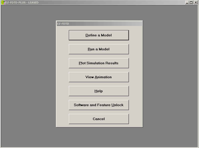
You can start EZ-EMC and EZ-FDTD by selecting it from the programs menu (once EZ-EMC or EZ-FDTD have been installed.) Once the ‘nag' screens are finished, select ‘Run EZ-EMC' or 'Run EZ-FDTD', and the general menu will appear (Figure 1). To create a model, press ‘Define a Model'. Note: the nag screens only appear for unlicensed versions, such as the demo version downloadable from the web page. Once the software has been purchased, a license file will be sent to the user which will stop the nag screens.
Figure 1
Build a Model
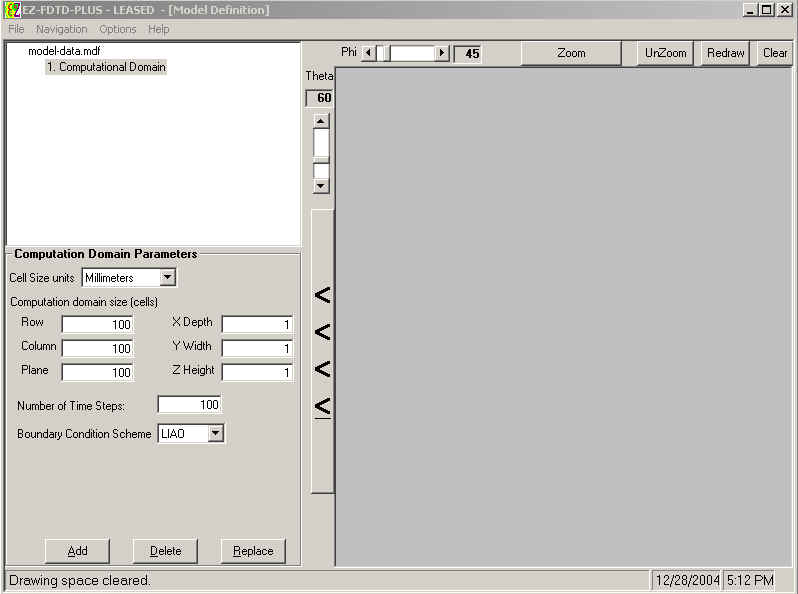
Once the ‘Define a Model' button has been pressed, the Model Definition window will appear (Figure 2). Before a FDTD model can be created, a computational domain must be created (ALL model features must exist within the computational domain). The Computational Parameters tree branch allows the user to select the FDTD cell size and the number of cells in each direction, for the computational domain.
Figure 2
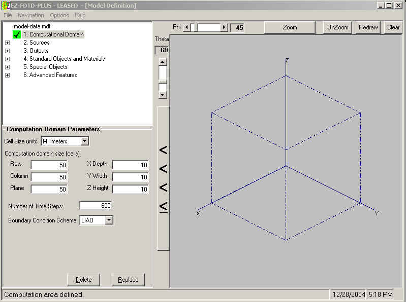
For this example, let's set the FDTD cell size to 10 mm (0.01 meters) in the x, y, and z directions. Let's set the computational domain to be 50 cells in each direction. Also, at this time, we'll set the number of time steps in the model to be 600. Figure 3 shows the drawing space once the ‘Add' button is pressed. The box represents the computational domain. Note that the view can be zoomed, and rotated in Theta and Phi using the controls at the upper left side of the drawing space, as shown in Figure 3a.
EZ-FDTD allows the user to select the absorbing boundary condition (ABC) scheme as Liao, PML or Mur. EZ-EMC has only Liao ABCs. Users who are not familiar with ABCs are urged to use the default Liao ABC in EZ-FDTD unless they have sufficient experience to understand the differences between ABCs.
Figure 2
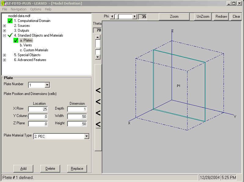
Note that once the ‘Add' button was pressed, the other model definition tree branches appeared below the computational parameters branch. Expand the 'Standard Objects and Materials' branch (by clicking on the '+' sign next to the 'Standard Objects and Materials' branch), and then select the ‘Plate' branch. We will create the plate halfway across the computational domain in the x direction. We will set the plate to start in the lower corner, and go to the upper corner, completely cutting the domain into two domains, keeping x=25 cells). (Note: this is allowed with the Liao absorbing boundary condition used in EZ-EMC and EZ-FDTD. Bringing a plate directly against the ABC simulates a plate to infinity in that direction.) We'll set the plate thickness to be 1 cell, and the plate material to be Perfect Electrical Conductor (PEC). PEC is a good approximation, since we expect the metal plate to be greater than a few skin depths, and so all the energy from one side to the other will be through the aperture. Figure 4 shows the drawing with the plate. The outline of the plate is shown, allowing a view to any objects ‘behind' the plate.
Figure 4
Next select the ‘Vents' branch. We'll select the aperture to be 10 cells by 2 cells and horizontally directed. We must select the x-direction start to be the same as the plate (25) and it's depth to be the same as the plate (1). We'll set the aperture in the center of the plate, as shown in Figure 5.
Figure 5

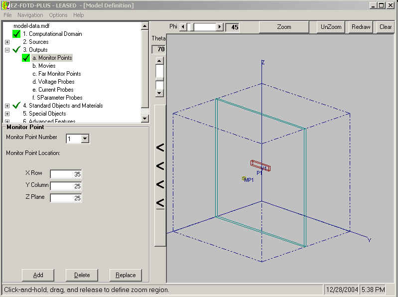
Next, we must put a source on one side, and a monitor point on the other side of the plate. Let's place the monitor point first, by expanding the 'Outputs' branch, and selecting the ‘Monitor point' branch. We simply use the cell coordinates to define where the monitor point is positioned. In this case, let's put a monitor point 10 cells from the aperture and centered on the aperture. Figure 6 shows the result once the monitor point has been ‘added'.
Figure 6
Note: most of the forms have a 'Replace' button. If you add an object, hole, source, etc. and then wish to change it, you can make the changes and use the 'Replace' button to update the model.
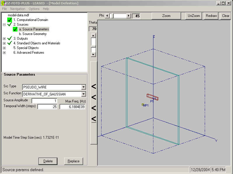
For the source, we must first set the type of source by expanding the 'sources' branch, and selecting the ‘Source Parameters' branch. Let's use the pseudo-wire and the derivative-of-Gaussian pulse. (Note: when using a pseudo-wire source, you must use the derivative-of-Gaussian pulse.) The source amplitude is selected as 1 for easy normalization later (if desired). The pulse width is set to 25 time steps. The pulse width controls the frequency domain content of the time domain pulse. A wider pulse has more low frequency content, and narrower pulse has more high frequency content. Figure 7 shows this view. At this time, there is no change to the drawing area. Note that the maximum frequency contained in the source pulse to 60 dB down from the peak amplitude is shown (in this case) to be ~ 6.2 GHz. The time step is also displayed after the 'Source Parameters' have been added.
Figure 7
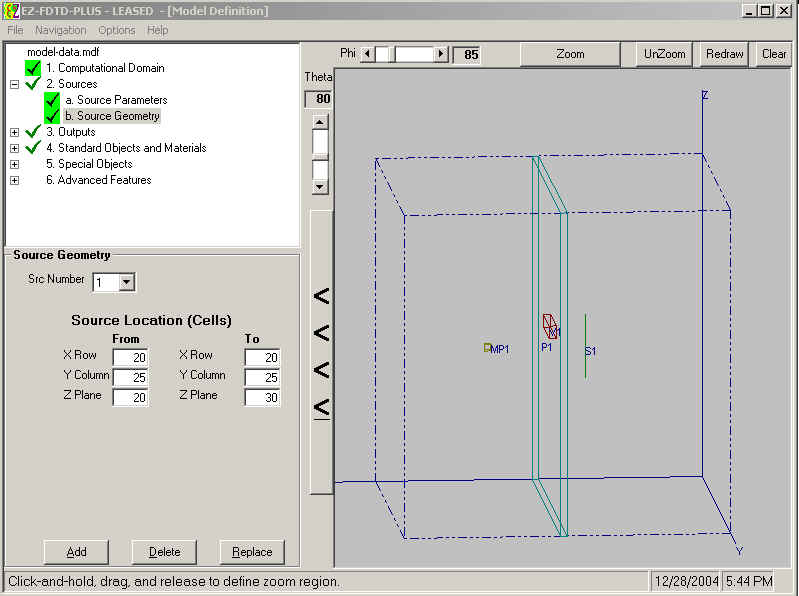
To finish specifying the source, we must specify the geometry by selecting the ‘Source Geometry' branch. We specify the source's location using cells. Let's create a source that is vertically polarized to optimize the emissions through the aperture. So, we'll select the source geometry as shown in Figure 8. Note the view has been rotated for easier viewing.
Figure 8
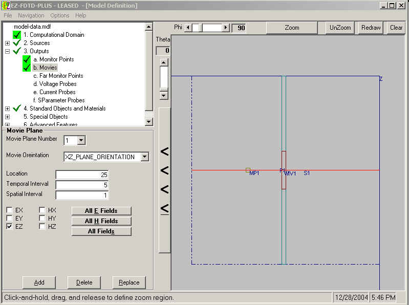
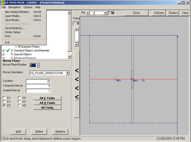
At this point, we could run the model. But first, let's set a movie plane so a animated movie will be saved. Expand the 'Outputs' branch, and select the ‘Movie' branch. As many movies as desired may be selected. Figure 9 shows a top-view of the model showing the movie plane cutting through the center of the model and including the aperture. The size of the resulting movie file can be quite large. Since the fields do not change rapidly with time, the temporal interval can be set to 5, without loss of viewing data, and only 1-in-5 time steps will be saved. The spatial interval is set to one, in this example, for a fine resolution movie. If the computational domain was much larger, the spatial interval could be raised to save disk space.
Figure 9
The model must be saved to an input file. Use the ‘File' pull down menu to save the model as example01.mdf. (Figure 9)
Figure 9
Run a Model
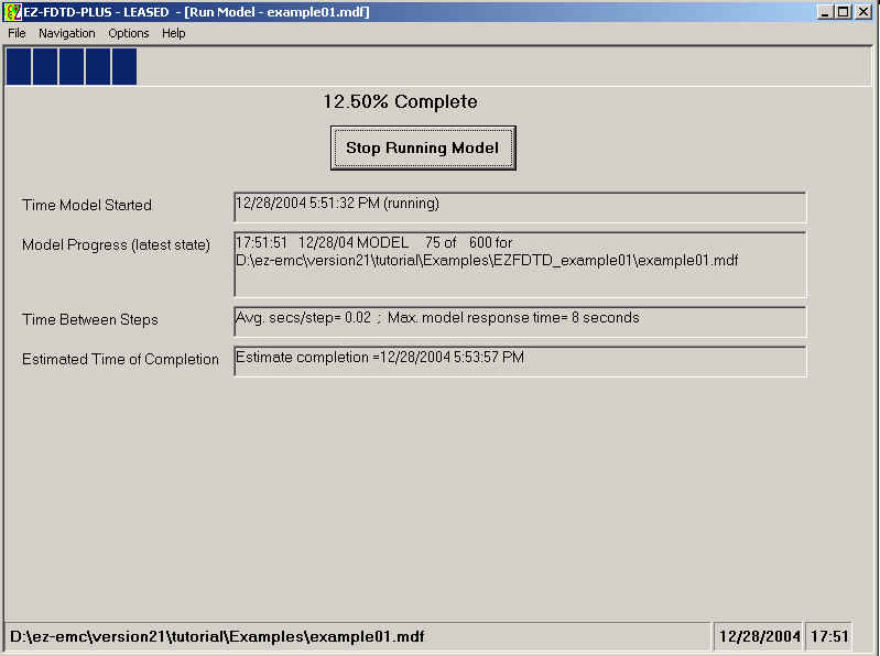
At this point, it is time to run the model. Select ‘Run a Model' from the ‘Navigation' pull down menu. Then select the file to run (example01.mdf) from the ‘File' pull down menu, select ‘open model and run'. Figure 10 shows the running model window display during the model run. A progress bar shows the percent complete, and an estimated time of completion is shown. If the model requires more RAM memory than present on the computer, a warning will be shown.
Figure 10
Plot Simulation Results
Once the model has finished running (100% complete indication), then select the ‘Plot Simulation Results' option from the ‘Navigation' pull down menu. Select the ‘open file' from the ‘File' pull down menu, and select the directory where the output files are located (not the output files themselves). Note: EZ-EMC and EZ-FDTD will create an output directory called EZEMC_example01 (or EZFDTD_example01) under the directory where the original input file is located. All output files will be in this new directory.
On the left side of the screen, click on the + sign next to Monitor Points to expand the list of monitor points. Then click on the + sign next to MP_1 to see the list of field orientations available. Double click on Ez to view the time domain view of the z-directed electric field as shown in Figure 11.
Figure 11

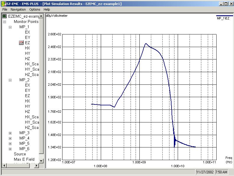
If frequency domain plots are desired, use the ‘Options' pull down menu, select ‘Plot by --- Frequency (Magnitude)'. The resulting plot is shown in Figure 12. Users may also plot the Frequency domain Phase, and a source-normalized magnitude plot.
Figure 12
If additional monitor points are available, they can be selected by simply expanding the field list for each desired monitor point, and double clicking on the desired field. Likewise, other files may be opened, and plotted on the same plot.
View Animation
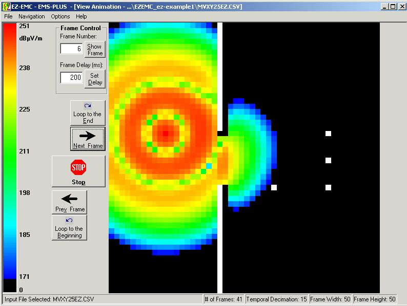
To see the animated movie of the fields, select ‘View Animation' from the ‘Navigation' pull down menu. Then select the file to view from the open file option in the ‘File' pull down menu.
All movie files will be located in the output directory created by EZ-FDTD or EZ-EMC. Movie files will start with the letters “MV”, then indicate the movie plane (e.g. XY), the location (e.g. 25), and the field, (e.g. EZ). For the example created above, the movie file name will be MXZ25EZ.csv. 'XZ' since the movie plane was the X-Z plane, '25' since the location of the movie plane was at y=25, and 'EZ' since this is the z-directed electric field. The movie can be single-stepped, or run repeatedly by using the buttons along the left side of the drawing area. Figure 13 shows an example of the movie display at a single time step.
Figure 13
Summary
This tutorial is intended to get a new person started quickly, using EZ-FDTD and/or EZ-EMC. There are a number of other options and features that are not discussed in this tutorial, but can be seen in the User's Manual. The users manual is available either as a standard alone HTML document, or as part of the integrated help within EZ-FDTD and EZ-EMC.